|
|
|
|
1
|
|
2
|
|
3
|
Click Add.
|
|
4
|
Click
|
|
5
|
In the Select Study tree, select Preset Studies for Selected Physics Interfaces>Time Dependent with FFT.
|
|
6
|
Click
|
|
1
|
|
2
|
|
1
|
|
2
|
|
3
|
|
1
|
|
2
|
|
3
|
|
1
|
|
2
|
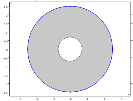
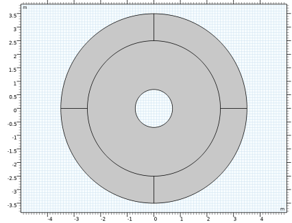
Select the object c1 only.
|
|
3
|
|
4
|
|
5
|
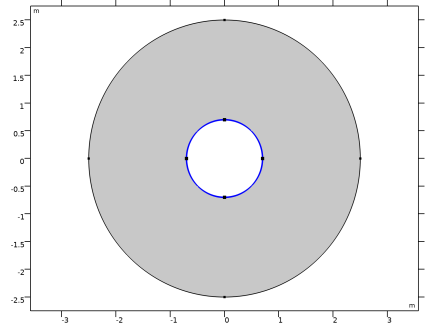
Select the object c2 only.
|
|
6
|
|
1
|
In the Model Builder window, under Component 1 (comp1) click Electromagnetic Waves, Time Explicit (ewte).
|
|
2
|
|
3
|
|
1
|
|
3
|
|
4
|
|
5
|
|
6
|
|
1
|
|
1
|
In the Model Builder window, expand the Far-Field Domain 1 node, then click Far-Field Calculation 1.
|
|
1
|
In the Model Builder window, under Component 1 (comp1) right-click Materials and choose Blank Material.
|
|
2
|
|
1
|
|
2
|
|
3
|
|
1
|
|
2
|
|
3
|
Click the Custom button.
|
|
4
|
|
5
|
|
1
|
|
2
|
|
3
|
In the Output times text field, type range(0,1/(4*fb0),10*T0). The Sampling rate 4*fb0 satisfies the Nyquist condition for the time to frequency fast Fourier transform (FFT) where its bandwidth is 2*fb0 excluding negative frequencies.
|
|
1
|
|
2
|
|
3
|
In the End time text field, type 20*T0. This makes sure that the FFT end time is longer than the simulation time so zero-padding can be applied during the time to frequency FFT. This will generate a finer frequency resolution in the resulting frequency response.
|
|
4
|
|
1
|
|
2
|
|
3
|
In the Excluded if text field, type freq<0.1*fb0 || freq>2*fb0-0.1*fb0. This excludes the first 5% and last 5% of the frequency response after FFT.
|
|
4
|
|
1
|
|
2
|
|
3
|
|
4
|
|
5
|
|
1
|
|
2
|
|
3
|
|
4
|
|
5
|
|
1
|
|
2
|
|
3
|
|
4
|
|
5
|
|
1
|
|
2
|
|
3
|
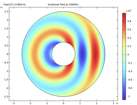
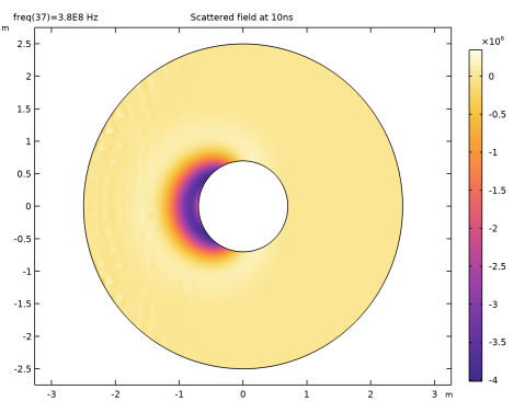
In the Expression text field, type Ez. This dependent variable is the z-component of the scattered field.
|
|
4
|
|
1
|
|
2
|
|
3
|
|
4
|
|
5
|
|
6
|
|
1
|
|
2
|
|
3
|
In the Expression text field, type ewte.Ez-ewte.Ebz. This is the difference in z-components between the total field and background field.
|
|
4
|
|
5
|
|
6
|
Click OK.
|
|
7
|
|
1
|
|
2
|
|
3
|
|
4
|
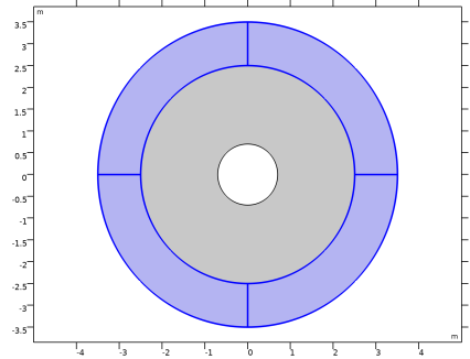
Click to expand the Layers section. In the table, enter the following settings:
|
|
5
|
|
6
|
|
1
|
|
3
|
|
4
|
|
1
|
In the Model Builder window, under Component 1 (comp1)>Electromagnetic Waves, Time Explicit (ewte) click Background Field 1.
|
|
1
|
|
2
|
|
3
|
Find the Studies subsection. In the Select Study tree, select Preset Studies for Selected Physics Interfaces>Time Dependent with FFT.
|
|
4
|
|
5
|
|
1
|
|
2
|
|
1
|
|
2
|
|
3
|
|
4
|
|
1
|
|
2
|
|
3
|
|
4
|
|
1
|
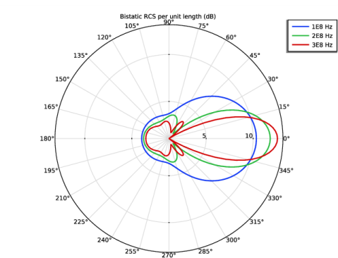
In the Model Builder window, under Results>Polar Plot Group 1 right-click Radiation Pattern 1 and choose Duplicate.
|
|
2
|
|
3
|
|
4
|
|
5
|
|
1
|
|
2
|
|
3
|
|
1
|
|
2
|
|
3
|
|
5
|
Locate the Coloring and Style section. Find the Line style subsection. From the Line list, choose Dashed.
|