PDF

Lossy Circular Waveguide
Introduction
In mode analysis it is usually the primary goal to find a propagation constant. This quantity is often, but not always, real valued; if the analysis involves some lossy part, such as a nonzero conductivity or an open boundary, the eigenvalue is complex. In such situations, the real and imaginary parts have separate interpretations:
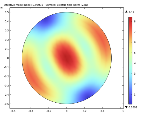
The imaginary part is the attenuation constant, measuring the damping in space
Model Definition
The mode analysis study for electromagnetic waves solves the eigenvalue problem
where
is the eigenvalue. For time-harmonic problems, the electric field for out-of-plane propagation can be written as
where z is the known out-of-plane direction.
The spatial parameter, α = δz + jβ = −λ, can have a real part and an imaginary part. The propagation constant is equal to the imaginary part, and the real part, δz, represents the damping along the propagation direction.
Variables influenced by mode Analysis
The following table lists the variables that are influenced by the mode analysis in terms of the eigenvalue lambda:
This two-dimensional model finds the modes of a circular waveguide with walls made of a nonperfect conductor, which is copper in this case. The losses in the walls lead to attenuation of the propagating wave. The propagation constant β is obtained as the imaginary part of α = − λ and the damping δz is obtained as the real part. Since the wave in the waveguide is attenuated in the z direction as e−δzz, the attenuation in dB scale is calculated using the formula
Results and Discussion
The eigenvalue solver returns six eigenvalues. Table 1 shows the six effective mode indices, neff, closest to 1, where
and k0 is the wave number in vacuum. The table also lists the propagation constant and damping in dB/m for each eigenmode.
The default surface plot shows the norm of the electric field for the effective mode index 0.9308 − 2.208·106j. This plot is shown in Figure 1.
Figure 1: The surface plot visualizes the norm of the electric field for the effective mode index 0.9308 - 2.208·10-6j.
Application Library path: RF_Module/Transmission_Lines_and_Waveguides/lossy_circular_waveguide
Modeling Instructions
From the File menu, choose New.
New
In the New window, click  Model Wizard.
Model Wizard
1
In the Model Wizard window, click  2D.
2
In the Select Physics tree, select Radio Frequency>Electromagnetic Waves, Frequency Domain (emw).
3
Click Add.
4
Click  Study.
5
In the Select Study tree, select Preset Studies for Selected Physics Interfaces>Mode Analysis.
6
Geometry 1
Circle 1 (c1)
1
In the Geometry toolbar, click  Circle.
2
In the Settings window for Circle, locate the Size and Shape section.
3
In the Radius text field, type 0.5.
4
Click  Build All Objects.
Add Material
1
In the Home toolbar, click  Add Material to open the Add Material window.
2
Go to the Add Material window.
3
4
Click Add to Component in the window toolbar.
Materials
Air (mat1)
By default the first material you add apply for all domains.
Next, specify copper as the material on the boundaries.
Add Material
1
Go to the Add Material window.
2
In the tree, select Built-in>Copper.
3
Click Add to Component in the window toolbar.
4
In the Home toolbar, click  Add Material to close the Add Material window.
Materials
Copper (mat2)
1
In the Settings window for Material, locate the Geometric Entity Selection section.
2
From the Geometric entity level list, choose Boundary.
3
From the Selection list, choose All boundaries.
Electromagnetic Waves, Frequency Domain (emw)
Impedance Boundary Condition 1
1
In the Model Builder window, under Component 1 (comp1) right-click Electromagnetic Waves, Frequency Domain (emw) and choose the boundary condition Impedance Boundary Condition.
2
In the Settings window for Impedance Boundary Condition, locate the Boundary Selection section.
3
From the Selection list, choose All boundaries.
Mesh 1
1
In the Model Builder window, under Component 1 (comp1) click Mesh 1.
2
In the Settings window for Mesh, locate the Physics-Controlled Mesh section.
3
In the table, clear the Use check box for Electromagnetic Waves, Frequency Domain (emw).
Solve for the 6 effective mode indices closest to 1.
Study 1
Step 1: Mode Analysis
1
In the Model Builder window, under Study 1 click Step 1: Mode Analysis.
2
In the Settings window for Mode Analysis, locate the Study Settings section.
3
Select the Desired number of modes check box.
4
In the Home toolbar, click  Compute.
Results
Electric Field (emw)
The default plot shows the electric field norm for the lowest mode found; compare with Figure 1.
Calculate the propagation constant and the attenuation constant (in dB) for each effective mode index.
Global Evaluation 1
1
In the Results toolbar, click  Global Evaluation.
2
In the Settings window for Global Evaluation, click Replace Expression in the upper-right corner of the Expressions section. From the menu, choose Component 1 (comp1)>Electromagnetic Waves, Frequency Domain>Global>emw.beta - Propagation constant - rad/m.
3
Click  Evaluate.
Compare the results with those in the second column of Table 1.
4
Click Replace Expression in the upper-right corner of the Expressions section. From the menu, choose Component 1 (comp1)>Electromagnetic Waves, Frequency Domain>Global>emw.dampzdB - Attenuation constant per meter, dB - dB/m.
5
Click  Evaluate.
Compare with the third column of Table 1.