Ion Drift Velocity Benchmark

When ions are subjected to a static electric field in a rarefied buffer gas, the combined effect of the electric force and collisions between the ions with ambient gas molecules causes the average ion velocity to approach an equilibrium value known as the ion drift velocity. The ability to accurately predict the drift velocity is important for the operation of devices such as ion mobility spectrometers, which are capable of accurately analyzing gas mixtures containing many different ion species by sorting the different species based on small variations in their drift velocity.

In this example, the average drift velocity of a group of argon ions is computed and compared to experimental data. The ions are modeled using the Charged Particle Tracing interface. Collisions with a neutral background gas are applied using the node, which supports various stochastic collision models including collisions and reactions. The resulting average ion drift velocity and ion temperature agree closely with values from the literature.

Model Definition

In this example, the model particles are Ar+ ions that are released in a neutral background gas of Ar atoms of a specified temperature and number density. The objective is to determine the average steady-state velocity, or drift velocity, of the ions under the combined influence of the continuous electric force and discrete collisions with the neutral atoms in the background gas.

The following sections provide an overview of the electric force definition and the theory of Monte Carlo collision modeling with the Charged Particle Tracing interface. For more information on the way random collisions are modeled with the Particle Tracing Module, see the section on Theory for the Charged Particle Tracing interface in the Particle Tracing Module Users’s Guide.

Electric Force

This model uses a over the electric field amplitude to analyze its effect on the ion drift velocity. Rather than being specified directly, the electric field amplitude is expressed in terms of the ratio E/N in Townsend units, where E (SI unit: V/m) is the amplitude of the electric field and N (SI unit: 1/m3) is the background gas number density. The Townsend unit is defined as 1 Td = 10−21 V m2. In this example, the is run from a minimum of E/N = 500 Td to a maximum of E/N = 105 Td.

The electric force Fe (SI unit: N) on each particle is simply

where e = 1.602176565 × 10-19 C is the elementary charge and Z (dimensionless) is the charge number. In this example Z = 1.

Collision Types

For the range of energies considered in this benchmark model, the interaction between the simulated Ar+ ions and the rarefied background gas of neutral Ar atoms is dominated by the following two reaction types:

collisions, in which only momentum is exchanged between the model particle and the neutral background argon atom, while the total kinetic energy is conserved; and

reactions, in which both charge and momentum are exchanged between the model particle and the background gas, typically resulting in a fast moving neutral atom and an slow-moving ion.

Collision Frequency and Collision Probability

Collisions between the argon ions and the neutral atoms occur at random times based on the total collision frequency ν(t) (SI unit: 1/s). given by the expression

where νj(t) is the collision frequency associated with the jth reaction in the model. In this example, j = 1 denotes the collision while j = 2 denotes the reaction.

In general the collision frequency associated with a specific collision type is

(1)

where

•

vg (SI unit: m/s) is the velocity of an atom or molecule in the background gas,

•

v (SI unit: m/s) is the particle velocity,

•

σj (SI unit: m2) is the collision cross section associated with the jth reaction, and

•

n (SI unit: 1/m3) is the number density of the gas.

The collision cross section for each reaction type can be an arbitrary function of the relative velocity and is usually determined experimentally. In this example the collision cross section is approximated as a function of energy using functions, although it can also be interpolated from imported tables of data with the function type.

The probability P(t) (dimensionless) that a particle undergoes a collision in a time interval (0, t) is

(2)

For constant collision frequency, Equation 2 simplifies to

(3)

Collision Detection Algorithms

The node in the Charged Particle Tracing interface provides two distinct algorithms for detecting and applying the random collisions between model particles and the atoms or molecules in a rarefied background gas. The choice of algorithm is controlled by the list, which has options , and .

Collision at Time Steps Taken by the Solver

The default option is a brute force approach that checks for collisions for each model particle at each time step taken by the solver. The following assumptions are made:

The collision frequency for each model particle is assumed constant over the following time step taken by the solver, even if the particle is accelerating.

Each model particle can undergo at most one collision per time step taken by the solver, which is applied at the beginning of the step.

Both assumptions 1 and 2 restrict the size of the time step taken by the solver for the results to be meaningful. The step size must be significantly smaller than the average free time between collisions, which might increase very rapidly if the particles are ions or electrons subjected to a strong electric field.

For each particle, a uniformly distributed random number U is sampled from the interval (0, 1). Then, because the collision frequency is assumed constant over the time step taken by the solver, the logical expression for a collision occurring is obtained by comparing U to the probability from Equation 3,

(4)

where some simplification has been made by noting that the probability distribution functions of U and 1 − U are exactly the same.

The pseudorandom number U is sampled once for every particle at the beginning of every time step taken by the solver.

Null Collision Method, Cold Gas Approximation

The option is an attempt to improve on the option by allowing multiple collisions to occur for each particle within a single time step taken by the solver and allowing these collisions to occur at distinct times between the discrete time steps.

The “cold gas approximation” is the omission of the gas velocity term vg from Equation 1,

This collision detection algorithm only applies to highly energetic particles, those that move at significantly higher speeds than the thermal speed of the background gas.

This algorithm is called the “null collision method” because the general approach is to overestimate the collision probability over a given time interval, predict collisions based on this overestimate of the collision frequency, and then discard a fraction of collisions based on the extent to which the real frequency is less than this artificial constant value, with these discarded interactions being called “null collisions”. Assume a constant trial frequency νm, such that νm > ν(t) over the time interval (0, t). If this trial frequency were the actual collision frequency over the time step, then Equation 3 would apply,

For each model particle, a trial time tm (SI unit: s) is computed such that Pm(tm) = U1, where U1 is a uniformly distributed number in the interval (0, 1) that is uniquely sampled for each particle. Solving for the trial time yields

Now that the trial times for each particle have been computed, a second uniformly distributed random number U2, not correlated with U1, is also randomly sampled from the interval (0, 1) for each particle that undergoes a collision in the time interval (0, t). If the inequality

(5)

holds true, then the collision is actually a null collision, and must be discarded.

The first integral in Equation 5 can be computed exactly, because the trial frequency is constant, but that the second integral can only be approximated numerically because the real collision frequency can be an arbitrary function of time. Therefore the size of the time step taken by the solver still has some bearing on the accuracy of the solution, even if this source of error is usually not as large as it is for the option .

Choosing Between Collision Types

For either collision detection algorithm, it is then necessary to determine whether the detected collision is of the elastic or resonant charge exchange variety. The probability pj of a specific collision type occurring is

where the denominator is, as usual, the total collision frequency over all collision types.

Reducing Simulation Time with a Stop Condition

The solver sequence in this example uses a to terminate the study when the particles have undergone a sufficient number of collisions. The rationale behind specifying a stop condition based on the maximum number of collisions over all particles, is that the maximum time needed for the average ion velocity to reach steady state may vary by several orders of magnitude over the parametric sweep of different electric field amplitudes. Thus, simply running the simulation to the same maximum solution time for every parameter value would be either wasteful for those parameter values that statistically converge most quickly, or inaccurate for those that statistically converge too slowly.

To keep track of the total number of collisions that each particle undergoes, the check box is selected in the settings for the node. The total number of collisions over all model particles is computed using the expression comp1.cpt.cptop1(comp1.cpt.col1.cex1.Nc). Here cpt.cptop1() is a built-in nonlocal coupling that computes the sum of an expression over all model particles.

Results and Discussion

The relationship between the reduced electric field magnitude and the average ion drift velocity is shown in Figure 1. The average ion temperature is shown in Figure 2.

In both plots, the computed solution shows good agreement with experimental data from Ref. 1.

Figure 1: Plot of the drift velocity of Ar+ ions in a background gas of neutral argon. The average drift velocity is compared to experimental data.

Figure 2: Plot of the ion temperature of Ar+ ions in a background gas of neutral argon. The average ion temperature is compared to experimental data.

Reference

1. A.V. Phelps, “Cross Sections and Swarm Coefficients for Nitrogen Ions and Neutrals in N2 and Argon Ions and Neutrals in Ar for Energies from 0.1eV to 10keV,” J. Phys. Chem. Ref. Data, vol. 20, no. 3, pp. 557–573, 1991.

2. A.V. Phelps, “The application of scattering cross sections to ion flux models in discharge sheaths,” J. Appl. Phys. vol. 76, pp. 747–753, 1994.

Particle_Tracing_Module/Charged_Particle_Tracing/ion_drift_velocity_benchmark

Modeling Instructions

From the menu, choose .

New

In the window, click

Model Wizard

In the window, click

In the tree, select .

Click .

Click

In the tree, select .

Click

Global Definitions

Parameters 1

In the window, under click .

In the window for , locate the section.

In the table, enter the following settings:


Name	Expression	Value	Description
mAr	0.04[kg/mol]/N_A_const	6.6422E-26 kg	Ar+ ion mass
ND	3.2956e22[1/m^3]	3.2956E22 1/m³	Background gas number density
EoverN	500	500	Reduced electric field in Townsend
Ez	1e-21[Vm^2]EoverN*ND	16478 V/m	Electric field magnitude
T0	300[K]	300 K	Gas temperature
maxCol	1e5	1E5	Maximum number of collisions for termination

Definitions

Enter raw data from Ref. 1 for the ion drift velocity as a function of the reduced electric field for elastic collisions between Ar+ ions and neutral Ar atoms.

Interpolation 1 (int1)

In the toolbar, click

and choose .

In the window for , locate the section.

From the list, choose .

Click

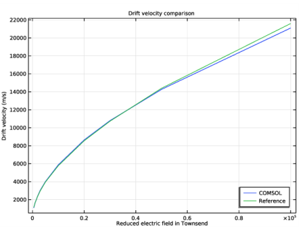
Browse to the model’s Application Libraries folder and double-click the file ion_drift_velocity_benchmark_velocity.txt.

Click

Locate the section. In the table, enter the following settings:


Function	Unit
Vdrift	m/s

Locate the section. In the text field, type Vdrift.

Interpolation 2 (int2)

Enter raw data from Ref. 1 for the ion temperature (eV) as a function of the reduced electric field.

In the toolbar, click

and choose .

In the window for , locate the section.

From the list, choose .

Click

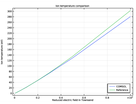
Browse to the model’s Application Libraries folder and double-click the file ion_drift_velocity_benchmark_temperature.txt.

Click

Locate the section. In the table, enter the following settings:


Function	Unit
ionTemp	eV

Locate the section. In the text field, type ionTemp.

Enter the analytic approximation for momentum cross section for elastic scattering between Ar+ ions and neutral Ar atoms from Ref. 2, which depends on the kinetic energy of the particles.

Analytic 1 (an1)

In the toolbar, click

and choose .

In the window for , type Qm in the text field.

Locate the section. In the text field, type 1.15e-18*x^(-0.1)*(1+0.015/x)^0.6.

Locate the section. In the table, enter the following settings:


Argument	Unit
x	eV

In the text field, type m^2.

Analytic 2 (an2)

Enter the analytic approximation for isotropic elastic collision between Ar+ ions and neutral Ar atoms from Ref. 2, which depends on the kinetic energy of the particles.

In the toolbar, click

and choose .

In the window for , type Qi in the text field.

Locate the section. In the text field, type 2e-19/(x^(0.5)*(1+x))+3e-19*x/(1+x/3)^(2.3).

Locate the section. In the table, enter the following settings:


Argument	Unit
x	eV

In the text field, type m^2.

Geometry 1

Cylinder 1 (cyl1)

In the toolbar, click

In the window for , locate the section.

In the text field, type 2.

In the text field, type 3.

Click

Charged Particle Tracing (cpt)

Particle Properties 1

In the window, under click .

In the window for , locate the section.

In the mp text field, type mAr.

Locate the section. In the Z text field, type 1.

Wall 1

In the window, click .

In the window for , locate the section.

From the list, choose .

Release from Grid 1

In the toolbar, click

and choose .

In the window for , locate the section.

In the qz,0 text field, type 1.

Locate the section. From the list, choose .

In the Nv text field, type 30.

In the T0 text field, type T0.

Electric Force 1

In the toolbar, click

and choose .

In the window for , locate the section.

From the list, choose .

Locate the section. Specify the E vector as


0	x
0	y
Ez	z

Collisions 1

In the toolbar, click

and choose .

In the window for , locate the section.

From the list, choose .

Locate the section. In the Nd text field, type ND.

In the T text field, type T0.

From the list, choose .

Locate the section. Select the check box.

Elastic 1

In the toolbar, click

and choose .

In the window for , locate the section.

In the σ text field, type Qi(cpt.Ep).

Locate the section. Select the check box.

Collisions 1

In the window, click .

Resonant Charge Exchange 1

In the toolbar, click

and choose .

In the window for , locate the section.

In the σ text field, type (Qm(cpt.Ep)-Qi(cpt.Ep))/2.

Locate the section. Select the check box.

Mesh 1

In the window, under right-click and choose .

Study 1

Parametric Sweep

In the toolbar, click

Sweep the reduced electric field from 500 Td to 1e5 Td.

In the window for , locate the section.

Click

In the table, enter the following settings:


Parameter name	Parameter value list	Parameter unit
EoverN (Reduced electric field in Townsend)	5e2, 1e3, 2e3, 3e3, 5e3, 1e4, 2e4, 3e4, 5e4, 1e5

Step 1: Time Dependent

To accurately predict the collisions, specify a maximum time and a manual time step size that are proportional to sqrt(maxCol/EoverN), which in turn is roughly proportional to the free time between collisions.

In the window, click .

In the window for , locate the section.

In the text field, type 0,5.0e-8*sqrt(maxCol/EoverN).

Solution 1 (sol1)

In the toolbar, click

In the window, expand the node, then click .

In the window for , click to expand the section.

From the list, choose .

In the text field, type 2.5e-9*sqrt(maxCol/EoverN).

In the text field, type 1.

Right-click and choose .

Set the stop condition to stop the time-dependent solver when the maximum number of collisions is reached. Make sure to store the solution at the time steps before and after the stop condition is fulfilled.

In the window for , locate the section.

Click

In the table, enter the following settings:


Stop expression	Stop if	Active	Description
comp1.cpt.sum(comp1.cpt.col1.cex1.Nc)>maxCol	True (>=1)	√	Stop expression 1

Locate the section. From the list, choose .

In the toolbar, click

Results

Drift Velocity

In the toolbar, click

and choose .

Compare the drift velocity to the tabulated data. Make this comparison at the last time step, after the drift velocity has reached an equilibrium value.

In the window for , type Drift Velocity in the text field.

Locate the section. From the list, choose .

From the list, choose .

Locate the section. From the list, choose .

Global 1

Right-click and choose .

In the window for , locate the section.

In the table, enter the following settings:


Expression	Unit	Description
cpt.ave(cpt.vz)	m/s
Vdrift(EoverN)	m/s

Locate the section. From the list, choose .

From the list, choose .

In the text field, type EoverN.

Click to expand the section. From the list, choose .

In the table, enter the following settings:


Legends
COMSOL
Reference

Drift Velocity

In the window, click .

In the window for , locate the section.

Select the check box. In the associated text field, type Drift velocity (m/s).

Click to expand the section. From the list, choose .

In the text area, type Drift velocity comparison.

In the toolbar, click

. The resulting image should look like Figure 1.

Ion Temperature

Now compare the ion energy to tabulated data. From Ref. 1, the average ion energy corresponds to a one dimensional energy distribution, that is, Ep = kBT/(2e).

Right-click and choose .

In the window for , type Ion Temperature in the text field.

Global 1

In the window, expand the node, then click .

In the window for , locate the section.

In the table, enter the following settings:


Expression	Unit	Description
cpt.ave(2*cpt.Ep)	eV
ionTemp(EoverN)	eV

Ion Temperature

In the window, click .

In the window for , locate the section.

In the text field, type Ion temperature (eV).

Locate the section. In the text area, type Ion temperature comparison.

In the toolbar, click

. The resulting image should look like Figure 2.