|
|
|
|
•
|
mphopen to load the model *.mph file.
|
|
•
|
mpheval to evaluate the outlet temperature at the mesh node points.
|
|
•
|
mphinterp to evaluate the outlet temperature at specified points.
|
|
•
|
mphplot to display plots.
|
|
1
|
Start COMSOL with MATLAB.
|
|
•
|
Enter each command, starting at step 2 below, at the MATLAB command line.
|
|
•
|
Paste the full model script, included in the section Model M-File, into a text editor, then save the file with a “.m” extension, and finally run this file in MATLAB.
|
|
4
|
Now add an interpolation function feature node named inletTemp to the model object. This reads the file pseudoperiodic_data.txt, which contains the temperature distribution at the outlet boundary. You generate the file under step 13 below. Type the following commands:
|
|
5
|
|
10
|
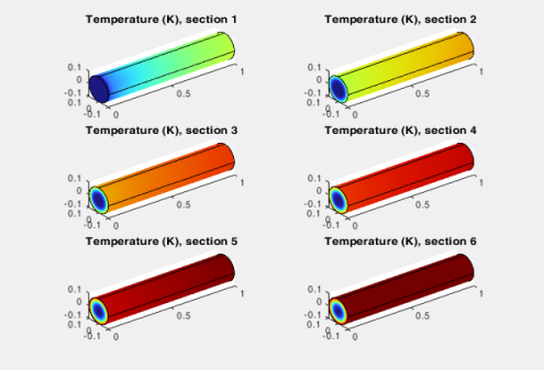
To display plot group pg2 enter:
|
|
11
|
Create a new MATLAB figure to display the plot group pg1 in a separate figure:
|
|
12
|
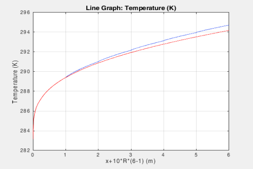
Next extract the temperature at the outlet boundary. Use the function mphinterp that requires that the coordinates for evaluation are defined in a mesh grid format. Enter the following commands:
|
|
13
|
|
1
|
First, re-initialize the inlet temperature condition to the constant value T0. Also, change the line color to red in the line graph. Type:
|
|
3
|
At the first iteration change the inlet temperature condition to inletTemp(x,y):
|
|
4
|
|
6
|
Next, plot the plot group pg1 in the second figure that has been generated in the previous loop (see step 11 on page 7), enter the commands below:
|
|
1
|
|
2
|
|
3
|
Click Add.
|
|
4
|
Click
|
|
5
|
|
6
|
Click
|
|
1
|
|
2
|
|
1
|
|
2
|
|
1
|
|
2
|
|
3
|
|
4
|
|
5
|
|
1
|
|
2
|
|
3
|
Click
|
|
1
|
|
2
|
|
3
|
Specify the u vector as
|
|
1
|
|
3
|
|
4
|
|
1
|
|
1
|
|
3
|
|
4
|
|
1
|
|
1
|
|
3
|
|
4
|
|
1
|
|
2
|
|
3
|
|
1
|
|
2
|
|
1
|
|
2
|
Browse to a directory which path is set in MATLAB and enter domain_activation_llmatlab in the File name text field.
|
|
3
|
Click Save.
|