|
|
|
|
•
|
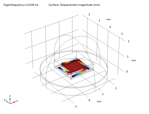
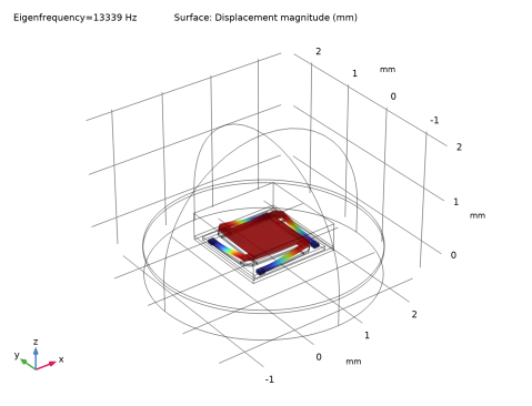
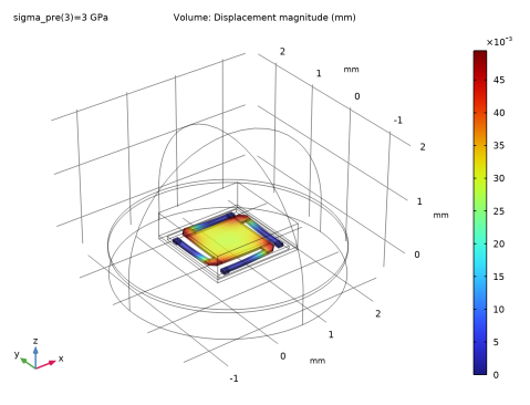
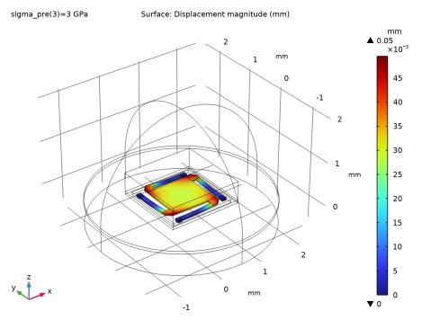
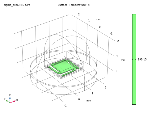
Thermoelasticity — to compute the mechanical losses from irreversible heat transfer driven by thermoelastic effect, which can be particularly important for small structures.
|
|
•
|
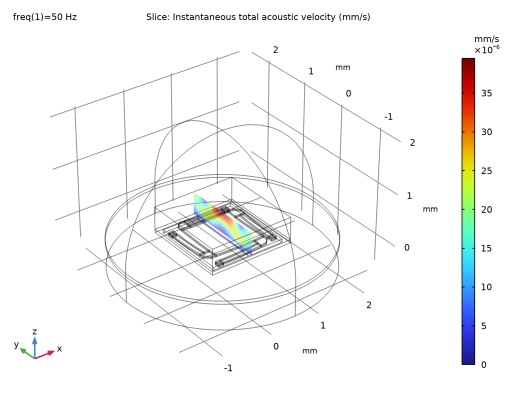
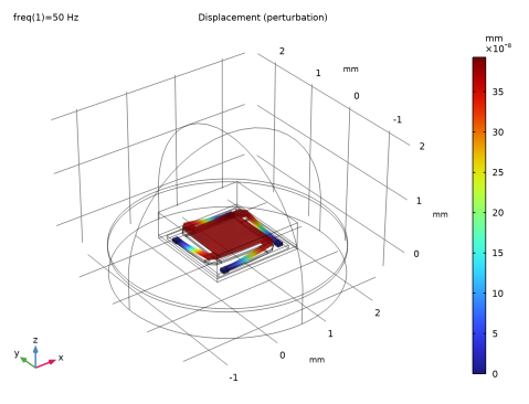
Thermoviscous Acoustics, Frequency Domain — to compute the acoustic variations of pressure, velocity, and temperature in geometries of small dimensions (microacoustics). This interface is used when modeling the response of transducers like microphones, miniature loudspeakers, and MEMS structures.
|
|
•
|
Pressure Acoustics, Frequency Domain — to compute the pressure variations for the propagation of acoustic waves in fluids at quiescent background conditions.
|
|
•
|
Thermal Expansion multiphysics coupling — to add an internal thermal strain caused by changes in temperature and account for the corresponding mechanical losses in the heat balance.
|
|
•
|
Thermoviscous Acoustics-Thermoelasticity Boundary multiphysics coupling — to model thermoviscous losses in acoustic-structure interaction problems to great detail. It captures the effect of a non-ideal thermal condition at the fluid-structure interface which is important in MEMS.
|
|
•
|
Acoustic-Thermoviscous Acoustic Boundary multiphysics coupling — to couple the Thermoviscous Acoustics interface to the Pressure Acoustics interface in both frequency and time domain.
|
|
•
|
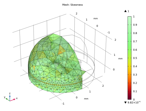
A box enclosing the original micromirror, assigned to the Thermoviscous Acoustics, Frequency Domain interface.
|
|
•
|
A half sphere surrounding the box, assigned to the Pressure Acoustics, Frequency Domain interface.
|
|
•
|
|
1
|
|
2
|
In the Select Physics tree, select Structural Mechanics>Thermal-Structure Interaction>Thermoelasticity.
|
|
3
|
Click Add.
|
|
4
|
In the Select Physics tree, select Acoustics>Thermoviscous Acoustics>Thermoviscous Acoustics, Frequency Domain (ta).
|
|
5
|
Click Add.
|
|
6
|
In the Select Physics tree, select Acoustics>Pressure Acoustics>Pressure Acoustics, Frequency Domain (acpr).
|
|
7
|
Click Add.
|
|
8
|
Click
|
|
9
|
In the Select Study tree, select Preset Studies for Selected Physics Interfaces>Solid Mechanics>Eigenfrequency, Prestressed.
|
|
10
|
Click
|
|
1
|
|
2
|
|
1
|
|
2
|
|
3
|
|
1
|
|
2
|
|
3
|
|
4
|
|
1
|
|
2
|
|
3
|
On the object sq2, select Point 4 only.
|
|
4
|
|
5
|
|
1
|
|
2
|
|
3
|
|
4
|
|
5
|
|
6
|
|
1
|
|
2
|
|
3
|
|
4
|
|
5
|
|
1
|
|
2
|
|
3
|
|
4
|
|
5
|
|
6
|
|
1
|
|
2
|
|
1
|
|
2
|
|
3
|
|
4
|
On the object ext1, select Boundaries 17, 26, 111, and 120 only.
|
|
5
|
Locate the Distances section. In the table, enter the following settings:
|
|
1
|
|
2
|
|
3
|
|
4
|
|
5
|
|
6
|
|
7
|
|
8
|
|
1
|
|
2
|
|
3
|
|
4
|
|
5
|
|
6
|
|
7
|
|
1
|
|
2
|
|
3
|
|
4
|
|
5
|
|
6
|
|
7
|
|
1
|
|
2
|
|
3
|
Select the object cyl2 only.
|
|
4
|
|
5
|
|
6
|
Select the object blk1 only.
|
|
1
|
|
2
|
|
3
|
|
4
|
|
5
|
|
6
|
|
7
|
|
8
|
|
1
|
|
2
|
|
3
|
|
4
|
|
5
|
|
6
|
|
1
|
|
2
|
|
3
|
|
1
|
|
2
|
Select the object sph1 only.
|
|
3
|
|
4
|
|
1
|
|
2
|
|
3
|
|
4
|
On the object par1, select Domain 1 only.
|
|
1
|
|
2
|
|
3
|
|
4
|
|
5
|
Click OK.
|
|
1
|
|
2
|
|
3
|
|
4
|
|
5
|
Click OK.
|
|
1
|
|
2
|
|
3
|
|
4
|
|
5
|
Click OK.
|
|
1
|
|
2
|
|
3
|
|
4
|
|
5
|
Click OK.
|
|
1
|
|
2
|
|
3
|
|
4
|
|
5
|
Click OK.
|
|
1
|
|
2
|
|
3
|
|
4
|
|
5
|
Click OK.
|
|
1
|
|
2
|
|
3
|
|
4
|
|
5
|
In the Paste Selection dialog box, type 24-28, 30, 31, 33, 34, 37-39, 41, 44, 47-52, 54, 55, 57, 58, 60-73, 75, 76, 78, 80-82, 84, 85, 87, 89-92, 94, 95, 98-106, 108, 109, 111, 113-115, 123, 124, 126, 128-130, 133-138, 140, 141, 143, 145-149, 152, 155, 157-162, 164, 165, 167, 168, 170-172, 174, 175, 178, 181-192 in the Selection text field.
|
|
6
|
Click OK.
|
|
1
|
|
2
|
|
3
|
|
4
|
|
5
|
Click OK.
|
|
1
|
|
2
|
|
3
|
In the tree, select Built-in>Aluminum.
|
|
4
|
|
5
|
|
6
|
|
7
|
In the tree, select Built-in>Air.
|
|
8
|
|
9
|
|
1
|
|
2
|
|
3
|
|
1
|
|
2
|
|
3
|
|
1
|
|
2
|
|
3
|
|
1
|
Right-click Global Definitions>Extra Dimension 1 (xdim1)>Mesh (Extra Dimension from Perfectly Matched Boundary 1) and choose Distribution.
|
|
3
|
|
4
|
|
1
|
In the Model Builder window, expand the Global Definitions>Extra Dimension 1 (xdim1)>Definitions>Extra Dimensions node, then click Points to Attach 1.
|
|
1
|
|
2
|
In the Settings window for Extra Dimension, type Extra Dimension from Perfectly Matched Boundary 1 in the Label text field.
|
|
3
|
|
4
|
Locate the Frames section. Find the Spatial frame coordinates subsection. In the table, enter the following settings:
|
|
5
|
|
6
|
|
7
|
|
1
|
|
2
|
|
3
|
|
4
|
|
5
|
Click OK.
|
|
6
|
|
7
|
|
1
|
|
2
|
|
3
|
|
4
|
|
5
|
|
6
|
|
7
|
Click OK.
|
|
8
|
|
9
|
|
1
|
|
2
|
|
3
|
|
4
|
|
5
|
|
6
|
Click OK.
|
|
7
|
|
8
|
|
1
|
|
2
|
|
3
|
|
4
|
|
5
|
Click OK.
|
|
1
|
|
2
|
|
3
|
|
4
|
|
5
|
Click OK.
|
|
6
|
|
7
|
|
8
|
|
9
|
|
10
|
|
1
|
|
2
|
|
3
|
|
1
|
|
2
|
|
3
|
|
4
|
|
5
|
Click OK.
|
|
1
|
In the Model Builder window, under Component 1 (comp1) click Thermoviscous Acoustics, Frequency Domain (ta).
|
|
2
|
In the Settings window for Thermoviscous Acoustics, Frequency Domain, locate the Domain Selection section.
|
|
3
|
|
4
|
|
5
|
Click OK.
|
|
6
|
In the Settings window for Thermoviscous Acoustics, Frequency Domain, locate the Domain Selection section.
|
|
7
|
|
8
|
|
9
|
Click OK.
|
|
10
|
In the Settings window for Thermoviscous Acoustics, Frequency Domain, locate the Domain Selection section.
|
|
11
|
|
12
|
|
13
|
|
14
|
|
15
|
Click OK.
|
|
1
|
|
2
|
|
3
|
|
4
|
|
5
|
Click OK.
|
|
6
|
|
7
|
|
8
|
|
1
|
In the Model Builder window, under Component 1 (comp1) click Pressure Acoustics, Frequency Domain (acpr).
|
|
2
|
In the Settings window for Pressure Acoustics, Frequency Domain, locate the Domain Selection section.
|
|
3
|
|
4
|
|
5
|
|
1
|
|
2
|
|
3
|
|
4
|
|
5
|
Click OK.
|
|
6
|
|
7
|
|
1
|
In the Model Builder window, under Component 1 (comp1)>Multiphysics click Thermal Expansion 1 (te1).
|
|
2
|
|
3
|
|
4
|
|
1
|
|
2
|
In the Settings window for Acoustic-Thermoviscous Acoustic Boundary, locate the Boundary Selection section.
|
|
3
|
|
1
|
|
2
|
In the Settings window for Thermoviscous Acoustic-Thermoelasticity Boundary, locate the Boundary Selection section.
|
|
3
|
|
1
|
|
2
|
|
3
|
|
4
|
In the Paste Selection dialog box, type 30, 37, 47, 60, 80, 89, 98, 113, 128, 145, 157, 170, 178 in the Selection text field.
|
|
5
|
Click OK.
|
|
1
|
|
2
|
|
3
|
|
4
|
|
5
|
In the Paste Selection dialog box, type 45, 115, 129, 134, 160, 173, 219, 304 in the Selection text field.
|
|
6
|
Click OK.
|
|
7
|
|
8
|
|
1
|
|
2
|
|
3
|
|
4
|
In the Paste Selection dialog box, type 56, 64, 74, 75, 95, 159, 199, 227, 243, 261, 288, 298 in the Selection text field.
|
|
5
|
Click OK.
|
|
6
|
|
7
|
|
1
|
|
2
|
|
3
|
|
4
|
|
5
|
Click OK.
|
|
6
|
|
7
|
|
1
|
|
2
|
|
3
|
|
4
|
|
1
|
|
2
|
|
3
|
|
4
|
|
1
|
|
2
|
|
3
|
|
4
|
|
5
|
|
6
|
Click OK.
|
|
7
|
|
1
|
|
2
|
|
3
|
Click the Custom button.
|
|
4
|
Locate the Geometric Entity Selection section. From the Geometric entity level list, choose Boundary.
|
|
5
|
|
6
|
|
7
|
Click OK.
|
|
8
|
|
9
|
|
1
|
|
2
|
|
3
|
Click the Custom button.
|
|
4
|
|
5
|
|
1
|
|
2
|
|
3
|
|
4
|
|
5
|
|
6
|
Click OK.
|
|
7
|
|
8
|
|
1
|
|
2
|
|
3
|
|
4
|
|
5
|
|
6
|
|
1
|
|
2
|
|
3
|
Click the Custom button.
|
|
4
|
|
5
|
|
6
|
|
1
|
|
2
|
In the Settings window for Study, type Study 1 - Structural Modes (lossless) in the Label text field.
|
|
3
|
|
1
|
|
2
|
|
5
|
Right-click Study 1 - Structural Modes (lossless)>Step 1: Stationary and choose Compute Selected Step.
|
|
1
|
|
2
|
|
3
|
|
4
|
|
5
|
|
6
|
|
8
|
|
1
|
|
2
|
|
3
|
Find the Studies subsection. In the Select Study tree, select Preset Studies for Selected Physics Interfaces>Solid Mechanics>Frequency Domain, Prestressed.
|
|
4
|
|
1
|
|
2
|
In the Settings window for Study, type Study 2 - Frequency Response: Full Model (ta-ht-solid) in the Label text field.
|
|
3
|
|
1
|
In the Model Builder window, under Study 2 - Frequency Response: Full Model (ta-ht-solid) click Step 1: Stationary.
|
|
2
|
|
3
|
|
4
|
Click
|
|
6
|
Right-click Study 2 - Frequency Response: Full Model (ta-ht-solid)>Step 1: Stationary and choose Compute Selected Step.
|
|
1
|
|
2
|
|
3
|
|
4
|
|
5
|
|
6
|
|
7
|
|
8
|
Click to expand the Values of Dependent Variables section. Find the Values of variables not solved for subsection. From the Settings list, choose User controlled.
|
|
9
|
|
10
|
|
11
|
|
1
|
|
2
|
Find the Studies subsection. In the Select Study tree, select Preset Studies for Selected Physics Interfaces>Solid Mechanics>Frequency Domain, Prestressed.
|
|
3
|
|
1
|
|
2
|
In the Settings window for Study, type Study 3 - Frequency Response Solid Losses (ht-solid) in the Label text field.
|
|
3
|
|
1
|
In the Model Builder window, under Study 3 - Frequency Response Solid Losses (ht-solid) click Step 1: Stationary.
|
|
2
|
|
4
|
|
5
|
Click
|
|
7
|
Right-click Study 3 - Frequency Response Solid Losses (ht-solid)>Step 1: Stationary and choose Compute Selected Step.
|
|
1
|
|
2
|
|
3
|
|
4
|
|
5
|
|
6
|
|
8
|
|
1
|
|
2
|
|
3
|
|
1
|
|
2
|
|
3
|
|
4
|
Click to expand the Selection section. Click to expand the Title section. Locate the Plot Settings section. Select the Propagate hiding to lower dimensions check box.
|
|
5
|
|
1
|
|
2
|
|
3
|
|
4
|
|
5
|
|
6
|
|
1
|
|
2
|
|
3
|
|
4
|
|
1
|
|
2
|
|
1
|
|
2
|
|
3
|
Locate the Data section. From the Dataset list, choose Study 2 - Frequency Response: Full Model (ta-ht-solid)/Solution Store 2 (sol4).
|
|
4
|
|
5
|
|
1
|
|
2
|
|
1
|
|
2
|
|
3
|
Locate the Data section. From the Dataset list, choose Study 2 - Frequency Response: Full Model (ta-ht-solid)/Solution Store 2 (sol4).
|
|
4
|
|
5
|
|
6
|
|
7
|
|
8
|
|
1
|
|
2
|
|
1
|
|
2
|
|
3
|
Locate the Data section. From the Dataset list, choose Study 2 - Frequency Response: Full Model (ta-ht-solid)/Solution Store 2 (sol4).
|
|
4
|
|
5
|
|
1
|
|
2
|
|
3
|
|
4
|
|
1
|
|
2
|
|
3
|
Locate the Data section. From the Dataset list, choose Study 2 - Frequency Response: Full Model (ta-ht-solid)/Solution 3 (sol3).
|
|
4
|
|
5
|
|
6
|
|
1
|
|
2
|
|
1
|
|
2
|
|
3
|
Locate the Data section. From the Dataset list, choose Study 2 - Frequency Response: Full Model (ta-ht-solid)/Solution 3 (sol3).
|
|
4
|
|
5
|
|
6
|
|
1
|
|
2
|
|
3
|
|
4
|
|
5
|
|
6
|
|
7
|
Click OK.
|
|
8
|
|
1
|
|
2
|
|
3
|
|
1
|
|
2
|
|
3
|
|
1
|
|
2
|
|
3
|
|
1
|
|
2
|
|
3
|
|
4
|
|
5
|
|
6
|
|
7
|
|
8
|
|
1
|
|
2
|
|
3
|
|
4
|
|
5
|
|
1
|
|
2
|
|
3
|
|
4
|
|
5
|
|
6
|
|
7
|
|
1
|
|
2
|
|
3
|
|
4
|
|
5
|
|
6
|
|
7
|
Click Define custom colors.
|
|
9
|
Click Add to custom colors.
|
|
10
|
|
1
|
|
2
|
|
3
|
|
4
|
|
5
|
Click OK.
|
|
1
|
|
2
|
|
3
|
|
4
|
|
5
|
|
6
|
|
1
|
|
2
|
|
3
|
|
4
|
|
5
|
|
1
|
|
2
|
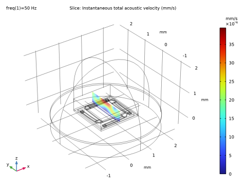
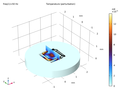
In the Settings window for 3D Plot Group, type Acoustic Velocity (perturbation) in the Label text field.
|
|
3
|
Locate the Data section. From the Dataset list, choose Study 2 - Frequency Response: Full Model (ta-ht-solid)/Solution 3 (sol3).
|
|
4
|
|
5
|
|
1
|
|
2
|
|
3
|
|
4
|
|
5
|
|
6
|
|
1
|
|
2
|
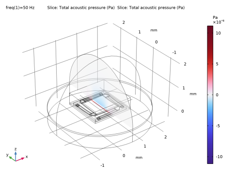
In the Settings window for 3D Plot Group, type Acoustic Pressure (perturbation) in the Label text field.
|
|
3
|
Locate the Data section. From the Dataset list, choose Study 2 - Frequency Response: Full Model (ta-ht-solid)/Solution 3 (sol3).
|
|
4
|
|
5
|
|
1
|
|
2
|
|
3
|
|
4
|
|
5
|
|
6
|
|
7
|
Click OK.
|
|
8
|
|
9
|
|
10
|
|
1
|
|
2
|
|
3
|
|
4
|
|
5
|
|
6
|
|
1
|
|
2
|
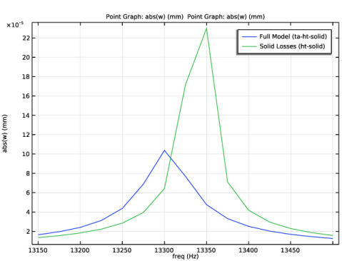
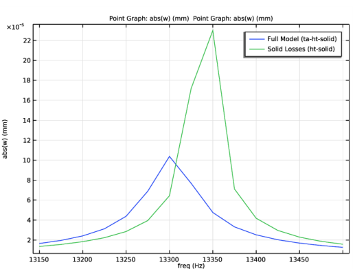
In the Settings window for 1D Plot Group, type Response Comparison (at resonance) in the Label text field.
|
|
3
|
Locate the Data section. From the Dataset list, choose Study 2 - Frequency Response: Full Model (ta-ht-solid)/Solution 3 (sol3).
|
|
4
|
|
5
|
|
1
|
|
2
|
|
3
|
|
4
|
|
5
|
Click OK.
|
|
6
|
|
7
|
|
8
|
|
9
|
|
10
|
|
12
|
|
1
|
|
2
|
|
3
|
From the Dataset list, choose Study 3 - Frequency Response Solid Losses (ht-solid)/Solution 5 (sol5).
|
|
4
|
|
5
|
|
6
|
Locate the Legends section. In the table, enter the following settings:
|
|
7
|
|
1
|
|
2
|
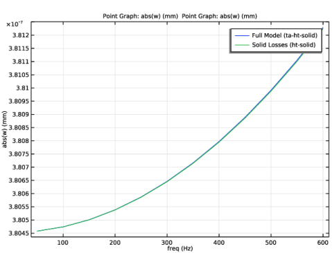
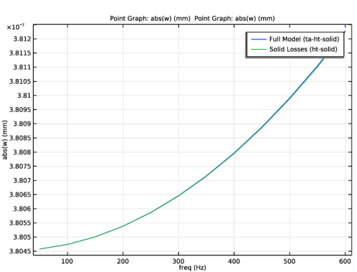
In the Settings window for 1D Plot Group, type Response Comparison (typical operation) in the Label text field.
|
|
3
|
Locate the Data section. From the Dataset list, choose Study 2 - Frequency Response: Full Model (ta-ht-solid)/Solution 3 (sol3).
|
|
4
|
|
5
|
|
1
|
|
2
|
|
3
|
|
4
|
|
5
|
Click OK.
|
|
6
|
|
7
|
|
8
|
|
9
|
|
10
|
|
12
|
|
1
|
|
2
|
|
3
|
From the Dataset list, choose Study 3 - Frequency Response Solid Losses (ht-solid)/Solution 5 (sol5).
|
|
4
|
|
5
|
|
6
|
Locate the Legends section. In the table, enter the following settings:
|
|
7
|